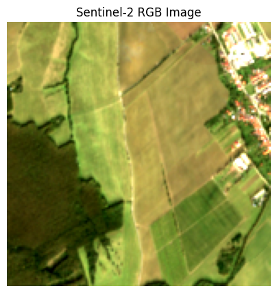
In this notebook, we perform dimensionality reduction on a full data cube of preprocessed Sentinel-2 satellite data. This data can quickly have many dimensions, consisting of many spectral bands, derived indexes and possibly other features, leading to very high-dimensional and heavy datasets. Working directly with such high-dimensional data presents several challenges:
Computational Efficiency: Lower-dimensional data requires less storage and speeds up downstream tasks like classification, clustering, or further processing.
Improved Visualization and Interpretation: By reducing dimensionality, we can visualize complex datasets in 2D or 3D plots, making it easier to understand underlying structures, patterns, or anomalies.
Curse of Dimensionality: As the number of features grows, the data becomes sparse in the feature space, making it harder to find meaningful patterns or clusters. Many machine learning algorithms also suffer performance drops or overfitting in very high dimensions.
Authentication
We first need to connect to an openEO provider. Most providers require you to register an account, and provide you with a basic amount of processing credits. In this notebook we will use the Copernicus Data Space Ecosystem as openEO provider.
All the known openEO providers and their services: https://hub.openeo.org/
More info on authentication: https://open-eo.github.io/openeo-python-client/auth.html
Run the authenticate_oidc() method again in case you can no longer connect. The token expires after a certain time.
This notebook will run two jobs: - One that select the significant raw bands from the dimensionality reduction model - One that executes the dimensionality reduction model
One model is applied, from scikit-learn, PCA. It is pre-trained with the same data we use in this notebook, to reduce all bands to 3 components.
It is recommended to zip your dependencies for scikit-learn, joblib & onnx since they differ vastly over the versions.
More info on scikit-learn PCA analysis: https://scikit-learn.org/stable/modules/generated/sklearn.decomposition.PCA.html
Load collection
We start off by loading in a collection. In this case, we are loading in Sentinel-2 L2A. More information on the collections available can be displayed with eoconn.list_collections(). Use eoconn.describe_collection("SENTINEL2_L2A") for example to get the description of a specific collection.
More information on finding and loading data: https://open-eo.github.io/openeo-python-client/data_access.html
For this exercise we use the derivatives of the 13 Sentinel-2 bands + NDVI by applying a spatial reduction - mean - median - max - min - q5 - q25 - q75 - q95
This leads to 112 (14x8) dimension to reduce in a dimensionality reduction model.
NDVI is added to indicate that either the source bands, B04 and B08 OR the NDVI will be used to determine significant bands by PCA loadings. It indicates that adding duplicate information has no effect in Dimensionality Reduction.
Load collection
data_cube = eoconn.load_collection("SENTINEL2_L2A", # or your collection id spatial_extent=BBOX, temporal_extent=[DATE_START, DATE_END], bands=['B01','B02','B03','B04','B05','B06','B07','B08','B8A','B09','B11','B12'], max_cloud_cover=10)
Temporally reduce data cube with different statistics
# Get original band labelsband_labels = data_cube_masked.metadata.band_names# Temporal reduce and prefix new band namesdef combined_reducer(t_array):""" Combined EO processes to reduce temporal resolution of an array """# Define every eo process mean = eop.mean(t_array) median = eop.median(t_array)min= eop.min(t_array)max= eop.max(t_array) q05 = eop.quantiles(t_array, probabilities=[0.05]) q25 = eop.quantiles(t_array, probabilities=[0.25]) q75 = eop.quantiles(t_array, probabilities=[0.75]) q95 = eop.quantiles(t_array, probabilities=[0.95])# Stack eo processes into arrayreturn eop.array_create([mean, median, min, max, q05, q25, q75, q95])# Now rename bands accordingly:target_bands = []for b in band_labels: target_bands.extend([f"{b}_mean", f"{b}_median", f"{b}_min", f"{b}_max",f"{b}_q05", f"{b}_q25", f"{b}_q75", f"{b}_q95" ])# Temporally reduce cube with combined reducer and rename bands accordinglysentinel_master_cube = data_cube_masked.apply_dimension( process=combined_reducer, dimension="t", target_dimension="bands").rename_labels("bands", target=target_bands)
Download RGB data from Sentinel-2 collection (mean value over spatial extent) to view
mean_bands = [b for b in sentinel_master_cube.metadata.band_names if b.endswith('_mean')]sentinel_mean_cube = sentinel_master_cube.filter_bands(mean_bands)sentinel_mean_cube.download(base_path /"mean_bands_cube.tiff")
Visualize RGB data
with rasterio.open(base_path /"mean_bands_cube.tiff") as src: pixel_size_x = src.transform.a pixel_size_y =-src.transform.eprint(f"Pixel Size: {pixel_size_x} x {pixel_size_y} units") r = src.read(4) # Band 3 g = src.read(3) # Band 2 b = src.read(2) # Band 1rgb = np.stack([r, g, b], axis=0)rgb_img = np.transpose(rgb, (1, 2, 0))# Normalize using percentilesdef normalize_percentile(img, lower=2, upper=98): p_low, p_high = np.percentile(img, (lower, upper)) img_clipped = np.clip(img, p_low, p_high)return (img_clipped - p_low) / (p_high - p_low)rgb_norm = normalize_percentile(rgb_img)plt.figure(figsize=(5, 5))plt.imshow(rgb_norm)plt.title("Sentinel-2 RGB Image")plt.axis("off")plt.show()
Pixel Size: 10.0 x 10.0 units
PCA model execution
Exploration of the data and the model
PCA characteristics: - Type: Linear - Objective: Find directions (principal components) that capture the maximum variance in the data. - Method: Eigen-decomposition of the covariance matrix. - Captures: Global structure in the data. - Output: Linear combinations of original features. - Interpretability: High (components are based on feature contributions). - Best for: Linearly structured data, noise reduction, feature compression, preprocessing for regression or classification.
When performing PCA, one of the key outputs is the Explained Variance Ratio. This metric tells us how much of the total variance in the original data is captured by each principal component. In other words, it helps us understand:
How many components are needed to retain most of the information (variance) in the data.
Which components are most informative, allowing us to reduce dimensionality effectively without losing essential structure.
Whether dimensionality reduction introduces significant information loss.
This makes the explained variance ratio a crucial diagnostic tool in PCA-based workflows, especially when deciding how many components to retain for visualization or modeling. Below you can find some model visualizations.
Explained Variance Ratio
This visualization helps understand how many principal components are needed to capture most of the variance in the data.
If the first few bars are tall and the rest are small, it means those components explain most of the variance, and dimensionality reduction can be effective.
ExplainedVarianceRatio.png
Cumulative Explained Variance
This plot helps you decide how many principal components to keep in your analysis by showing the cumulative amount of variance explained.
For example, if the curve reaches 90% explained variance at the 4th component, you might choose to keep only the first 4 components for dimensionality reduction, but this is now already reached with 3 components.
CumulativeExplainedVariance.png
Band Significance curve
This code helps identify which original spectral bands (features) are most influential in the PCA model by examining the loadings.
It filters out bands with insignificant contributions and visually ranks bands by their maximum contribution to any principal component.
This can guide to feature extraction, interpretation, or further analysis by focusing on the most important spectral bands.
Only bands with a loading of at least 0.01 are shown. You can see here while NDVI doesn’t reach this threshold, that its soucres bands B04 & B08 reach very high loadings.
BandSignificanceCurve.png
Significant Band Loadings Heatmap
This heatmap visually summarizes which spectral bands contribute strongly to which principal components and whether the contribution is positive or negative.
By filtering for significant bands, the plot focuses on the most meaningful relationships (weight > 0.20 for at least one of the components) in the PCA,
helping you interpret how each component is formed by combinations of original bands.
AbsoluteSignificantBandLoadingsHeatmap.png
UDF execution
UDF: select significant bands by pca loadings
Based on the previous curves we decide to only keep 18 bands (weight > 0.20 on the heatmap). The underlying UDF selects those features based on our PCA model.
In case you want to keep bands based on the loading, you can also give a threshold betweeen 0 and 1 of how big the loading needs to be.
Failed to parse API error response: [503] 'no available server\n' (headers: {'Content-Type': 'text/plain; charset=utf-8', 'X-Content-Type-Options': 'nosniff', 'Date': 'Fri, 31 Oct 2025 17:03:03 GMT', 'Content-Length': '20'})
0:01:57 Job 'j-25103117010540ffb02e0fdc90b9eed0': Service availability error while polling job status: [503] no available server

0:02:28 Job 'j-25103117010540ffb02e0fdc90b9eed0': running (progress N/A)
0:03:00 Job 'j-25103117010540ffb02e0fdc90b9eed0': running (progress N/A)
0:03:37 Job 'j-25103117010540ffb02e0fdc90b9eed0': running (progress N/A)
0:04:24 Job 'j-25103117010540ffb02e0fdc90b9eed0': running (progress N/A)
0:05:23 Job 'j-25103117010540ffb02e0fdc90b9eed0': finished (progress 100%)
WindowsPath('results/significant_bands.nc')
Check how many of the bands are reduced and left
# Open the NetCDF fileds = xr.open_dataset("results/significant_bands.nc")# Extract band variables, excluding 'crs'bands = [var for var in ds.data_vars if var !="crs"]# Print total countprint(f"{len(bands)} bands left:\n")# Print bands in a numbered listfor i, band inenumerate(bands, start=1):print(f"{i}. {band}")
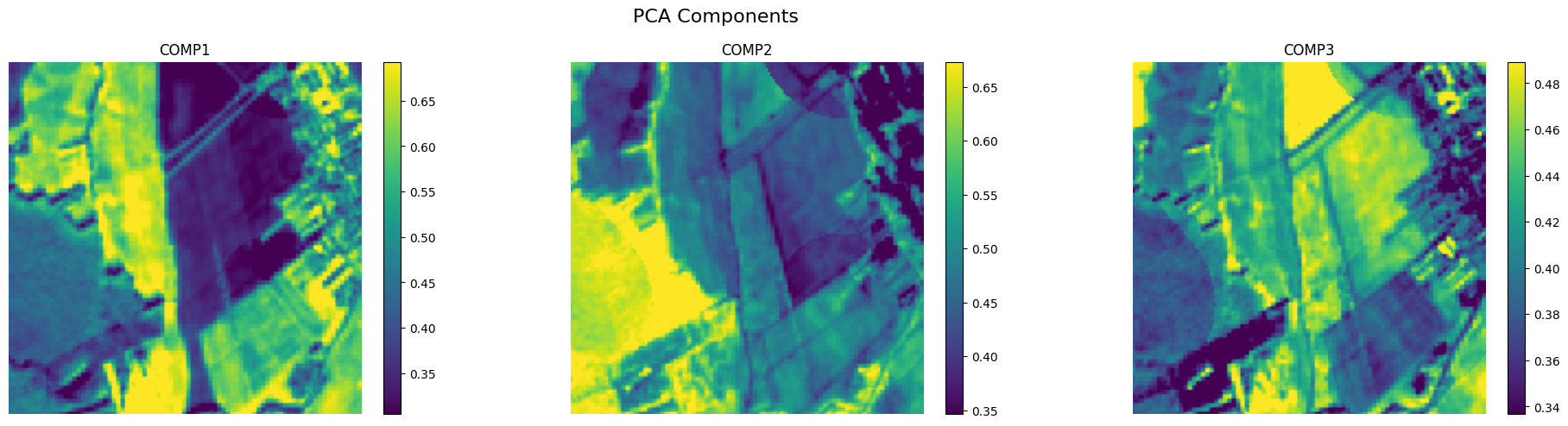
When performing dimensionality reduction on spatial data, the output components represent key underlying patterns or features extracted from the original dataset. Visualizing these components side-by-side helps reveal how different spatial structures contribute to the overall variability. By examining subtle variations in each component, we can better understand dominant spatial trends, detect anomalies, or identify meaningful features that may not be obvious in the raw data. Effective visualization with appropriate color scaling ensures these differences are clear and interpretable, aiding in model validation, feature extraction, and communication of results.
These new bands with the most important information, are not only easier easier to visualize and analyze, imaging plotting 141 bands, they could also be used in Machine-learning models as input bands.
def concat_features_to_bands_dim(ds: xr.DataArray):# List band variables band_vars = [var for var in ds.data_vars if ds[var].dtype.kind in'fc'andset(ds[var].dims) == {'y', 'x'}] cube = xr.concat([ds[var] for var in band_vars], dim="bands") cube = cube.assign_coords(bands=band_vars) # name the bandsreturn cube.rename('__xarray_dataarray_variable__')def plot_components(data_array: xr.DataArray, model_name: str): fig, axes = plt.subplots(1, 3, figsize=(20, 5))print(type(data_array))for i, ax inenumerate(axes): comp_data = np.abs(data_array.isel(bands=i)) # take absolute value here# Use percentiles to plot as vmin & vmax to highlight differences vmin = comp_data.quantile(0.05).item() vmax = comp_data.quantile(0.95).item() im = ax.imshow(comp_data, vmin=vmin, vmax=vmax) ax.set_title(f'COMP{i+1}') ax.axis('off') fig.colorbar(im, ax=ax, fraction=0.046, pad=0.04)# Add a general title fig.suptitle(f"{model_name} Components", fontsize=16) plt.tight_layout() plt.show()